We can port even more complicated problems from mathematics directly to a functional language. For an example closer to home, let us consider a binomial pricing model, illustrating that the ease and elegance with which Haskell handles factorial do indeed extend to real-life quantitative finance problems as well.
The binomial tree pricing model works by assuming that the price of an underlying asset can only move up or down by constant factors  and
and  during a small time interval
  . Stringing together many such time intervals, we make up the expiration time of the derivative instrument we are trying to price. The derivative defined as a function of the price of the underlying at any point in time.
 |
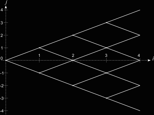
| Figure 1. Binomial tree pricing model. On the X axis, labeled i, we have the time steps. The Y axis represents the price of the underlying, labeled j. The only difference from the standard binomial tree is that we have let j be both positive and negative, which is mathematically natural, and hence simplifies the notation in a functional language. |
We can visualize the binomial tree as shown in Fig. 1. At time  , we have the asset price
  . At
. At  (with the maturity
  ). we have two possible asset values
  and
and  , where we have chosen
  . In general, at time
  , at the asset price node level
  , we have

By choosing the sizes of the up and down price movements the same, we have created a recombinant binomial tree, which is why we have only  price nodes at any time step
  . In order to price the derivative, we have to assign risk-neutral probabilities to the up and down price movements. The risk-neutral probability for an upward movement of
  is denoted by
  . With these notations, we can write down the fair value of an American call option (of expiry
  , underlying asset price
  , strike price
  , risk free interest rate
  , asset price volatility
  and number of time steps in the binomial tree
  ) using the binomial tree pricing model as follows:

where  denotes the fair value of the option at any the node
  in time and
  in price (referring to Fig. 1).

At maturity,  and
and  , where we exercise the option if it is in the money, which is what the first Max function denotes. The last term in the express above represents the risk neutral backward propagation of the option price from the time layer at
  to
to  . At each node, if the option price is less than the intrinsic value, we exercise the option, which is the second Max function.
The common choice for the upward price movement depends on the volatility of the underlying asset.  and the downward movement is chosen to be the same
  to ensure that we have a recombinant tree. For risk neutrality, we have the probability defined as:

For the purpose of illustrating how it translates to the functional programming language of Haskell, let us put all these equations together once more.

where


Now, let us look at the code in Haskell.
optionPrice t s0 k r sigma n = f 0 0
    where
      f i j =
          if i == n
          then max ((s i j) - k) 0
          else max ((s i j) - k)
                    (exp(-r*dt) * (p * f(i+1)(j+1) +
                    (1-p) * f(i+1)(j-1)))
      s i j = s0 * u**j
      u = exp(sigma * sqrt dt)
      d = 1 / u
      dt = t / n
      p = (exp(r*dt)-d) / (u-d)
As we can see, it is a near-verbatim rendition of the mathematical statements, nothing more. This code snippet actually runs as it is, and produces the result.
*Main> optionPrice 1 100 110 0.05 0.3 20
10.10369526959085
Looking at the remarkable similarity between the mathematical equations and the code in Haskell, we can understand why mathematicians love the idea of functional programming. This particular implementation of the binomial pricing model may not be the most computationally efficient, but it certainly is one of great elegance and brevity.
While a functional programming language may not be appropriate for a full-fledged implementation of a trading platform, many of its underlying principles, such as type abstractions and strict purity, may prove invaluable in programs we use in quantitative finance where heavy mathematics and number crunching are involved. The mathematical rigor enables us to employ complex functional manipulations at the program level. The religious adherence to the notion of statelessness in functional programming has another great benefit. It helps in parallel and grid enabling the computations with almost no extra work.
Sections

 and
and  during a small time interval
  . Stringing together many such time intervals, we make up the expiration time of the derivative instrument we are trying to price. The derivative defined as a function of the price of the underlying at any point in time.
 , we have the asset price
  . At
. At  (with the maturity
  ). we have two possible asset values
  and
and  , where we have chosen
  . In general, at time
  , at the asset price node level
  , we have
 price nodes at any time step
  . With these notations, we can write down the fair value of an American call option (of expiry
  , underlying asset price
  , strike price
  , risk free interest rate
  , asset price volatility
  and number of time steps in the binomial tree
  ) using the binomial tree pricing model as follows:
 denotes the fair value of the option at any the node
  in time and
 and
and  , where we exercise the option if it is in the money, which is what the first Max function denotes. The last term in the express above represents the risk neutral backward propagation of the option price from the time layer at
  to
to  and the downward movement is chosen to be the same


