
Nothing is certain but death and taxes, they say. On the death front, we are making some inroads with all our medical marvels, at least in postponing it if not actually avoiding it. But when it comes to taxes, we have no defense other than a bit of creativity in our tax returns.
Let’s say Uncle Sam thinks you owe him $75k. In your honest opinion, the fair figure is about the $50k mark. So you comb through your tax deductible receipts. After countless hours of hard work, fyou bring the number down to, say, $65k. As a quant, you can estimate the probability of an IRS audit. And you can put a number (an expectation value in dollars) to the pain and suffering that can result from it.
Let’s suppose that you calculate the risk of a tax audit to be about 1% and decide that it is worth the risk to get creative in you deduction claims to the tune of $15k. You send in the tax return and sit tight, smug in the knowledge that the odds of your getting audited are fairly slim. You are in for a big surprise. You will get well and truly fooled by randomness, and IRS will almost certainly want to take a closer look at your tax return.
The calculated creativity in tax returns seldom pays off. Your calculations of expected pain and suffering are never consistent with the frequency with which IRS audits you. The probability of an audit is, in fact, much higher if you try to inflate your tax deductions. You can blame Benford for this skew in probability stacked against your favor.
Skepticism
Benford presented something very counter-intuitive in his article [1] in 1938. He asked the question: What is the distribution of the first digits in any numeric, real-life data? At first glance, the answer seems obvious. All digits should have the same probability. Why would there be a preference to any one digit in random data?
Benford showed that the first digit in a “naturally occurring” number is much more likely to be 1 rather than any other digit. In fact, each digit has a specific probability of being in the first position. The digit 1 has the highest probability; the digit 2 is about 40% less likely to be in the first position and so on. The digit 9 has the lowest probability of all; it is about 6 times less likely to be in the first position.
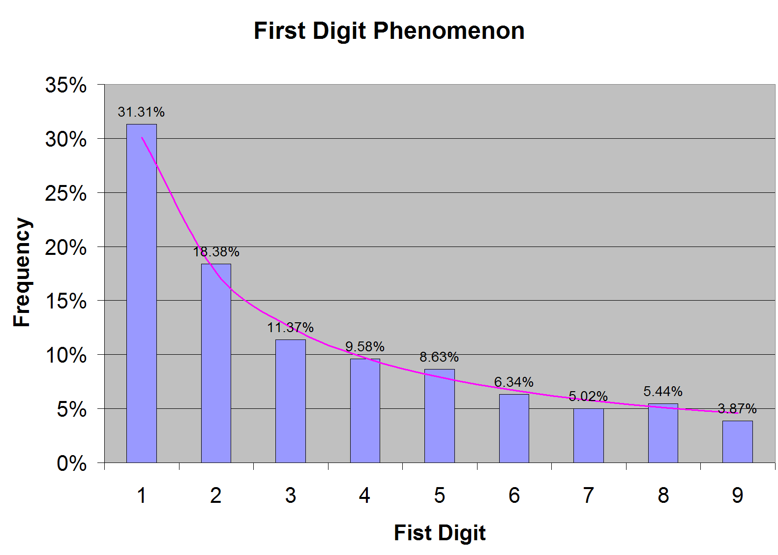
When I first heard of this first digit phenomenon from a well-informed colleague, I thought it was weird. I would have naively expected to see roughly same frequency of occurrence for all digits from 1 to 9. So I collected large amount of financial data, about 65000 numbers (as many as Excel would permit), and looked at the first digit. I found Benford to be absolutely right, as shown in Figure 1.
The probability of the first digit is pretty far from uniform, as Figure 1 shows. The distribution is, in fact, logarithmic. The probability of any digit d is given by log(1 + 1 / d), which is the purple curve in Figure 1.
This skewed distribution is not an anomaly in the data that I happened to look at. It is the rule in any “naturally occurring” data. It is the Benford’s law. Benford collected a large number of naturally occurring data (including population, areas of rivers, physical constants, numbers from newspaper reports and so on) and showed that this empirical law is respected.
Simulation
As a quantitative developer, I tend to simulate things on a computer with the hope that I may be able to see patterns that will help me understand the problem. The first question to be settled in the simulation is to figure out what the probability distribution of a vague quantity like “naturally occurring numbers” would be. Once I have the distribution, I can generate numbers and look at the first digits to see their frequency of occurrence.
To a mathematician or a quant, there is nothing more natural that natural logarithm. So the first candidate distribution for naturally occurring numbers is something like RV exp(RV), where RV is a uniformly distributed random variable (between zero and ten). The rationale behind this choice is an assumption that the number of digits in naturally occurring numbers is uniformly distributed between zero and an upper limit.
Indeed, you can choose other, fancier distributions for naturally occurring numbers. I tried a couple of other candidate distributions using two uniformly distributed (between zero and ten) random variables RV1 and RV2: RV1 exp(RV2) and exp(RV1+RV2). All these distributions turn out to be good guesses for naturally occurring numbers, as illustrated in Figure 2.
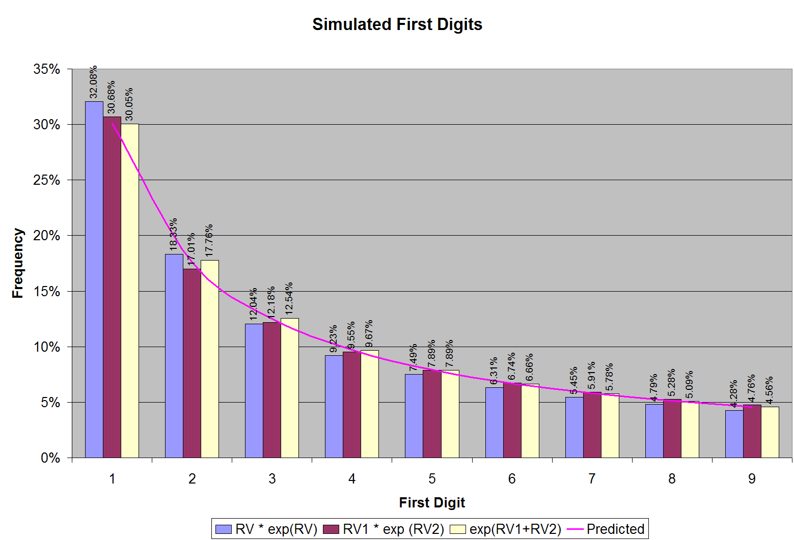
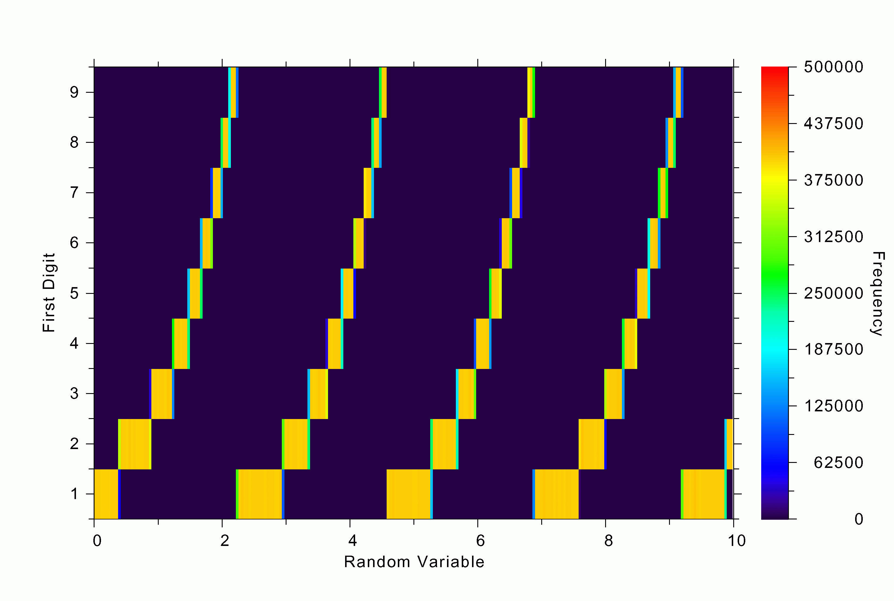
The first digits of the numbers that I generated follow Benford’s law to an uncanny degree of accuracy. Why does this happen? One good thing about computer simulation is that you can dig deeper and look at intermediate results. For instance, in our first simulation with the distribution: RV exp(RV), we can ask the question: What are the values of RV for which we get a certain first digit? The answer is shown in Figure 3a. Note that the ranges in RV that give the first digit 1 are much larger than those that give 9. About six times larger, in fact, as expected. Notice how pattern repeats itself as the simulated natural numbers “roll over” from the first digit of 9 to 1 (as an odometer tripping).
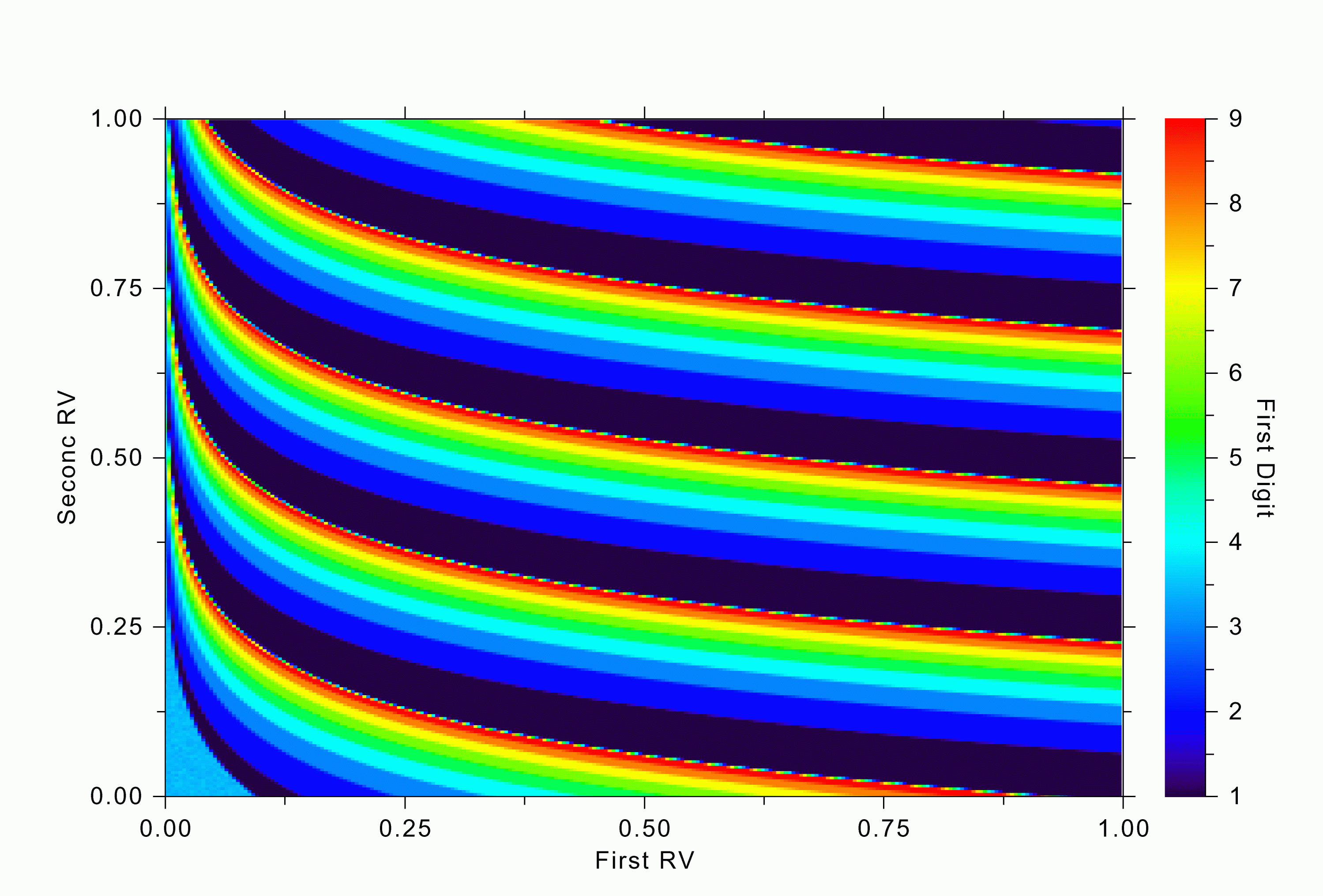
A similar trend can be seen in our fancier simulation with two random variables. The regions in their joint distributions that give rise to various first digits in RV1 exp(RV2) are shown in Figure 3b. Notice the large swathes of deep blue (corresponding to the first digit of 1) and compare their area to the red swathes (for the first digit 9).
This exercise gives me the insight I was hoping to glean from the simulation. The reason for the preponderance of smaller digits in the first position is that the distribution of naturally occurring numbers is usually a tapering one; there is usually an upper limit to the numbers, and as you get closer to the upper limit, the probably density becomes smaller and smaller. As you pass the first digit of 9 and then roll over to 1, suddenly its range becomes much bigger.
While this explanation is satisfying, the surprising fact is that it doesn’t matter how the probability of natural distributions tapers off. It is almost like the central limit theorem. Of course, this little simulation is no rigorous proof. If you are looking for a rigorous proof, you can find it in Hill’s work [3].
Fraud Detection
Although our tax evasion troubles can be attributed to Benford, the first digit phenomenon was originally described in an article by Simon Newcomb [2] in the American Journal of Mathematics in 1881. It was rediscovered by Frank Benford in 1938, to whom all the glory (or the blame, depending on which side of the fence you find yourself) went. In fact, the real culprit behind our tax woes may have been Theodore Hill. He brought the obscure law to the limelight in a series of articles in the 1990s. He even presented a statistical proof [3] for the phenomenon.
In addition to causing our personal tax troubles, Benford’s law can play a crucial role in many other fraud and irregularity checks [4]. For instance, the first digit distribution in the accounting entries of a company may reveal bouts of creativity. Employee reimbursement claims, check amounts, salary figures, grocery prices — everything is subject to Benford’s law. It can even be used to detect market manipulations because the first digits of stock prices, for instance, are supposed to follow the Benford distribution. If they don’t, we have to be wary.
Moral
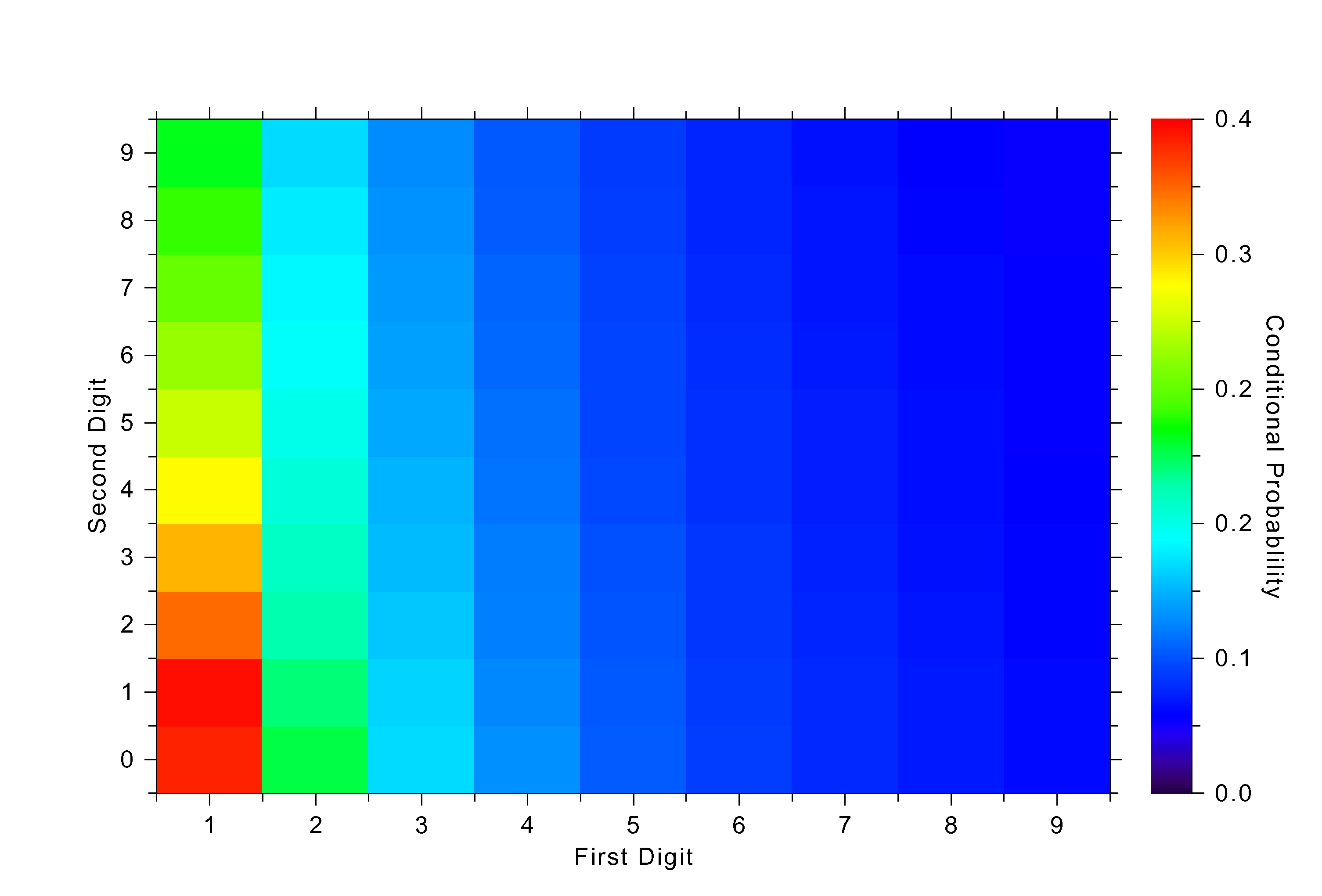
The moral of the story is simple: Don’t get creative in your tax returns. You will get caught. You might think that you can use this Benford distribution to generate a more realistic tax deduction pattern. But this job is harder than it sounds. Although I didn’t mention it, there is a correlation between the digits. The probability of the second digit being 2, for instance, depends on what the first digit is. Look at Figure 4, which shows the correlation structure in one of my simulations.
Besides, the IRS system is likely to be far more sophisticated. For instance, they could be using an advanced data mining or pattern recognition systems such as neural networks or support vector machines. Remember that IRS has labeled data (tax returns of those who unsuccessfully tried to cheat, and those of good citizens) and they can easily train classifier programs to catch budding tax evaders. If they are not using these sophisticated pattern recognition algorithms yet, trust me, they will, after seeing this article. When it comes to taxes, randomness will always fool you because it is stacked against you.
But seriously, Benford’s law is a tool that we have to be aware of. It may come to our aid in unexpected ways when we find ourselves doubting the authenticity of all kinds of numeric data. A check based on the law is easy to implement and hard to circumvent. It is simple and fairly universal. So, let’s not try to beat Benford; let’s join him instead.
References
[1] Benford, F. “The Law of Anomalous Numbers.” Proc. Amer. Phil. Soc. 78, 551-572, 1938.
[2] Newcomb, S. “Note on the Frequency of the Use of Digits in Natural Numbers.” Amer. J. Math. 4, 39-40, 1881.
[3] Hill, T. P. “A Statistical Derivation of the Significant-Digit Law.” Stat. Sci. 10, 354-363, 1996.
[4] Nigrini, M. “I’ve Got Your Number.” J. Accountancy 187, pp. 79-83, May 1999. http://www.aicpa.org/pubs/jofa/may1999/nigrini.htm.
Photo by LendingMemo